Symmetric polynomial map was first studied by K.Uchimura.
This map is defined by
X = x^2 + c y
Y = y^2 + c x
considred in the two dimensional complex space.
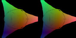
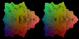
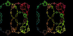
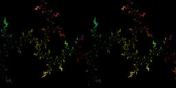
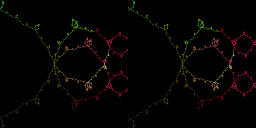
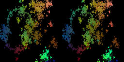
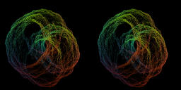
Itsu second Julia set is computed by taking a generic point and plotting many points of its backward images.
Each point of C^2 pas four points as its backward image( except critical points).
In the following movies,4^10 points are computed and projected into the real three dimensional space and plotted in a stereographic way.
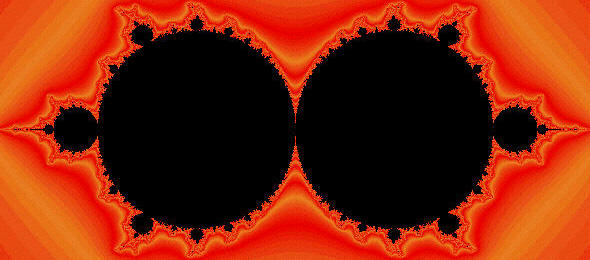 Double Mandelbrot set.
Parameters from left half of the double Mandelbrot set.
 For c=2.0[movie2-1]579KB, hypocycloid.
 For c=-2.01[movie2-2]1MB, Cantor set.
 For c=-1.99[movie2-3]650KB
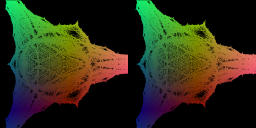 For c=-1.9[movie2-4]1.2MB, a space ship.
 For c=-0.6004851804+1.2496206i[movie2-5]1.2MB, a dendrite(?).
 For c=-0.5480566+0.95732930i[movie2-6]1.4MB, second Julia set for Douady's rabbit parameter.
 For c=-1.23606798[movie2-7]1.6MB, period two superattracting cycle.
 For c=-1[movie2-8]1.8MB, perod doubling parameter, parabolic basin.
 For c=1[movie2-9]317MB, saddle-node bifurcation, parabolic basin .
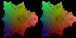
 For c=-2.2 to c=-0.2[movie2-10]5.7MB, metamorphose of second Julia sets.
Parameters from right half of the double Mandelbrot set.
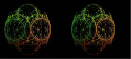
 For c=2[movie2-11]187KB, three cicles in the priodic complex lines and their backward images.
 For c=1.3[movie2-12]1.9MB, one dimensional Julia sets and their backward images.
 For c=2.5[movie2-13]897KB.
 For c=3.0[movie2-14]830KB, infinitely many copies of San Marco Juia sets.
 For c=4.0[movie2-15]613KB, Julia set in the invariant line and periodic lines are straight segemnts and their inverse images and the closure of them foem the second Julia set.
 For c=2.600485+1.24962166i[movie2-16]958KB,dendrite case.
 For c=2.54805+0.9573293i[movie2-17]991KB,Douady's rabbit case( one dimansional map has a superattractive cycle of period three ) .
 For c=3.236079[movie2-18]908KB, one dimensional dynamics has a superattractive cycle of period two.
 For c=2.8090-0.587785i[movie2-20]914KB,one dimensional map has a parabolic cycle of period 5.
 For c varied from 0.2 to 4.0[movie2-21]3.8MB, second Julia set transforms its shape from almost torus to dendrite via various fractal set.
Regular polynomial maps here are defined by
X = x^2 + a x + b y
Y = y^2 + c x + d y
 For a=0, b=1, c=-1, d=0.[Movie3-1][2.79MB]
 For a=-0.61607+0.455357i, b=1.205357-0.348214i, c=-0.455357-0.348242i, d=0.3482144-0.455357i.[Movie3-2][2.11MB]
 For a=0.7232144;0.133928i, b=0.8-0.9910714i, c=-1.098214+0.1i, d=0.0-0.455357i.[Movie3-3][2.43MB]
 For a=-0.61607;0.455357i, b=1.205357-1.3125i, c=-0.455357+1.473214i, d=0.348214387-1.258928i. [Movie3-4][2.86MB]
 For a=-0.6160714, b=0.401785, c=1.258928-0.40178579i, d=-1.5803570. [Movie3-5][1.83MB]
 For a=0.7232148+0.133928i, b=0.8, c=0.1i, d=0.2i. [Movie3-6][1.38MB]
 For a=0.12+0.74i, b=0.2i, c=0, d=0.25. This is a skew product case.[Movie3-7][1.81MB]
Regular polynomial maps (x,y) to (X,Y) here are defined by
u = x^2 + a x + b y
v = y^2 + c x + d y
X = p u + q v
Y = r u + s v
 Parameters are taken as
a=-0.8, b=0.8, c=0.1i, d=0.2i,p=s=1,q=r=0.
And c is varied to -2.9125, while other parameters are fixed.
[Movie3-8][5.3MB]
Parameters are taken as
a=-0.8, b=0.8, c=0.1i, d=0.2i,p=s=1,q=r=0.
And c is varied to -2.9125, while other parameters are fixed.
[Movie3-8][5.3MB]
 Initial parameters are same as the previous movie. They are moved to a=-0.8+0.723i,
b=-1.8445, c=-0.134+0.1i,d=-0.416i.[Movie3-9][9.6MB]
Initial parameters are same as the previous movie. They are moved to a=-0.8+0.723i,
b=-1.8445, c=-0.134+0.1i,d=-0.416i.[Movie3-9][9.6MB]
 Initial parameters are sams as above. Parameters are varied to p=-1.259,
q=0.884, r=-1.4196, s=1.0982.[Movie3-10][11MB]
Initial parameters are sams as above. Parameters are varied to p=-1.259,
q=0.884, r=-1.4196, s=1.0982.[Movie3-10][11MB]
 Initial parameters are a=-0.0268, b=-0.777, c=-0.7232-0.0248, d=0.13393i, p=s=1,q=r=0.
They are varied by a : -0.0804i, b : -0.0804, c:-0.02678,d:0.026785i,
p:-0.455357, q:-2.8125, r:3.0, s:-0.723214.[Movie3-11][4.7MB]
Initial parameters are a=-0.0268, b=-0.777, c=-0.7232-0.0248, d=0.13393i, p=s=1,q=r=0.
They are varied by a : -0.0804i, b : -0.0804, c:-0.02678,d:0.026785i,
p:-0.455357, q:-2.8125, r:3.0, s:-0.723214.[Movie3-11][4.7MB]
 Parameters are forgotten.[Movie3-12][7.7MB]
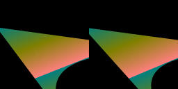 For c=-2.0[movie1-1]248KB, Flying triangle.
 For c=-2.2[movie1-2]1.5MB, Cantor triangle.
 For c=0.0[movie1-3]577KB, Moebius band case.
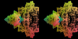 For c varied fron -2.0 to 0.05[movie1-4]8.3MB